Here I describe a fast filter-and-refine algorithm for finding interceptions of a sequence of Earth geodesic segments by a set of points, such as between a GPX file’s route and waypoints, which I developed last year for my open source project CoursePointer. [1] Combining this filter with Karney’s geodesic interception algorithm [9] yields precise points of interception while being simpler to implement than an R-tree—and probably more efficient for some common use cases, at the tradeoff of order of growth.
I’ve been unable to find this exact approach documented elsewhere, including by asking AI to help me search for prior art. If you’re aware of an earlier description that I’ve missed please email me and I’ll update this post!
Problem Statement and Background
Given a path as a sequence of geodesic segments on the WGS84 spheroid Earth model, plus a set of points on the spheroid, how can we quickly find where any of the points “intercept” the path within some threshold distance? [2]
Concretely, I wrote CoursePointer to convert GPX routes/tracks and waypoints into Garmin FIT course files and course points. [3] Waypoints and course points have different semantics: A waypoint is just a point somewhere on the spheroid, given as a latitude and longitude, which may or may not be located along a route or track in the same GPX file. A course point, on the other hand, is specifically associated with—and located at a certain distance along—a course. That distance is needed as part of its FIT representation.
So to generate course points, my program must answer the question: “Does this route ever get within e.g. 35 m of that waypoint? And if so, how far along the overall route does that happen?”
Figure 1: A route made of multiple segments, and some waypoints. Waypoint A is near to the route, so it should be interpreted as a course point along it; Waypoint B is far from the route and should not be considered a course point.
But how do we model these segments and waypoints? A 2D projection is easy for small areas, but as a general solution it introduces edge cases and distortions that require correction. A spherical Earth model is better but can still be off from the spheroid by around 0.5%. [8] For both precision and consistency with other GIS/GPS tools, I’d prefer to do these calculations on the WGS84 spheroid.
The interception of a geodesic segment from a point on the spheroid does not have a closed-form solution, but there are iterative methods. [9] [10] Karney’s method, which he also describes succinctly in a SourceForge comment, involves taking a gnomonic projection centered on a guess of the point of interception, using Cartesian geometry to compute a new guess, and iterating until the guess converges. This provides an accurate answer—but it’s not the fastest thing to do between every combination of route segment and waypoint in a GPX file.
So we need some filter to reject combinations of path segments and points that we can deduce must be outside of our interception threshold. R-trees and k-d-trees can efficiently query nearby objects, but these add complexity and take time to initialize, on top of which rectangular bounding boxes are suboptimal for path segments oriented in arbitrary directions. Given my project’s narrower requirements, I thought I could do something simpler—and maybe even faster, for the routes I’m interested in?
Typical Segment Lengths
My main interest lies in the sorts of routes exported from hiking or cycling planners, such as Gaia GPS, Komoot, or Ride with GPS. We can look at an example route to get a sense of the scale of typical route segments.
Opening this example road cycling route in Mathematica reveals 2209 segments (including some zero-length ones) with a median length of 40 m, a mean of 50 m, and a maximum of 303 m. Twistier hiking trails will tend to have still shorter segments.
Figure 2: A distribution of segment lengths from a real-world road cycling route.
This means it would be useful to have a filter capable of providing a tight bound on a waypoint’s distance from shorter segments, in particular.
CoursePointer’s Filter
CoursePointer’s filter establishes this tight lower bound by approximating segments with chords of WGS84. This dramatically reduces the amount of work needed in the part of the program, with being the number of segments and the number of waypoints.
The high-level approach is:
- Approximate each geodesic segment of the path with a chord of the spheroid between its endpoints. Also convert each waypoint into Euclidean space.
- Use Euclidean geometry, plus reasoning about how far a geodesic of that length may diverge from its chord, to establish a lower bound on the actual geodesic distance between each segment and waypoint.
- Reject segment-point combinations whose lower bound distances are higher than our interception threshold. For segment-point combinations potentially within our threshold, use Karney’s algorithm to precisely compute the geodesic interception and distance.
Segmentation and Conversion to Euclidean Space
We begin by segmenting the route, given as a sequence of route/track points, into adjacent pairs. (Some route planners may include some zero-length segments in the route, and we can exclude those for efficiency.) For each pair, we:
- Solve the inverse problem to obtain the geodesic distance between them. CoursePointer uses GeographicLib, which implements this in Geodesic::Inverse. [11]
- Convert each endpoint into 3D Euclidean space. This transformation uses the standard oblate spheroid coordinate formulas, and GeographicLib provides it as Geocentric::Forward.
We also convert all the waypoints into Euclidean space.
Figure 3: Segment endpoints and a waypoint represented as points in Euclidean space. These can also be considered as vectors extending from the center of the model. The two segment endpoints, and , implicitly define a chord between them.
Point-to-Chord Distance
For each waypoint and route segment we compare, we can then find the distance between the waypoint and the segment’s approximation chord in Euclidean space. We start by taking two new vectors:
Figure 4: Two new vectors and , based on subtracting from and from , respectively.
We want to know how far is from its nearest point along , as illustrated by the dashed line:
Figure 5: The distance and projection of from/onto .
It might be tempting to measure and then calculate , but that only works if we already know . Imagine combinations of segments and points where , which would bring the projection behind the start of the route segment; on the other hand, if is too long or is too small, the projection could extend beyond its end. Instead, we need to calculate the pictured vector which points somewhere along the chord, including its endpoints, but not beyond them.
To start with, consider the unbounded projection of onto the line extending through . We’ll call this :
Using the dot product identities and , this can be rewritten as:
We then only need to clamp to the extent of the chord. The full point–chord distance calculation becomes: [4]
In Rust, given appropriate vector types, this can be written as:
fn euclidean_intercept_distance<P>(
    segment: &GeoSegment<GeoAndXyzPoint>,
    point: &P,
) -> Result<Meter<f64>>
where
    P: HasXyzPoint,
{
    let b = segment.end.xyz() - segment.start.xyz();
    let a = point.xyz() - segment.start.xyz();
    Ok((a - euclidean_intercept(a, b)).norm())
}

fn euclidean_intercept<V: DisplacementVector>(a: V, b: V) -> V {
    let dot_ab = dot(a, b);
    if dot_ab <= 0.0 * M2 {
        V::zero() // Clamp to segment start
    } else {
        let dot_bb = dot(b, b);

        // dot(a, b) >= dot(b, b) iff a_proj.norm() >= b.norm()
        if dot_ab >= dot_bb {
            b // Clamp to segment end
        } else {
            b * (dot_ab / dot_bb) // a_proj
        }
    }
}
This works great in practice because it avoids trigonometry; the point-chord distance is calculated with just a handful of elementary floating-point operations. But this doesn’t yet constitute a lower bound on the actual geodesic distance between the waypoint and the segment.
Establishing the Lower Bound
In many cases the Euclidean distance between a waypoint and a segment’s approximation chord will be smaller than the geodesic distance from the actual segment, but this is not guaranteed. Consider:
Figure 6: A case where the point-segment geodesic distance is smaller than the vector distance to the approximation chord.
For one example, if the chord is long enough that its sagitta exceeds the actual point–segment distance, the point–chord distance fails to provide a lower bound. Additionally, the geodesic on a spheroid (unlike on a sphere) isn’t necessarily in a plane, and may further diverge toward the point along the surface.
Boissonnat, Lieutier, and Wintraecken (2019) [12] provide a general upper bound on the distance between a geodesic of this manifold and the chord between its endpoints:
Lemma 13: Let be such that and let be a minimizing geodesic parametrized by arc length connecting and with length , then
If we substitute the spheroid’s minimum radius of curvature for and take the worst case of the midpoint of the geodesic (where ), this reduces to
for . [5] And at Claude’s suggestion, by using the half-angle trigonometric identity that , we can further rewrite this to avoid excessive loss of floating-point precision on account of subtracting potentially tiny quantities from 1:
This suggests a very tight bound for real-world routes. A segment as long as 500 m (around the longest I’ve seen in practice, for my use case) has a of about 5 mm, and remains below 200 m even for hypothetical segments up to 100 km:
Figure 7: vs. the geodesic segment length for .
Filtering Stage
Now imagine a cylinder drawn around each of our segments’ chords. The radius of each is for that segment’s geodesic.
Figure 8: Cylinders around segment chords. Each segment’s actual geodesic lies within its cylinder of radius .
If our waypoint intercepts a segment’s geodesic somewhere nearer than it does its chord, that must happen within its cylinder, so provides a lower bound on the Euclidean distance between the point and the segment geodesic. And because the geodesic distance between any two points on the surface of the spheroid is no smaller than their Euclidean distance, this also provides a lower bound on the geodesic distance between the point and the segment, which is ultimately what we care about.
The filter is then:
- Calculate the distance between the waypoint and the segment’s chord.
- Subtract for that segment. [6]
- If greater than our interception threshold (e.g., 35 m), reject that waypoint-segment combination as “far away”.
Refinement and Interception
For waypoint-segment pairs not rejected by the filter we apply Karney’s geodesic interception algorithm. Each waypoint then has an associated, ordered list of segments like
| Segment | Distance |
|---|---|
| 1 | Far |
| 2 | Near(32 m) |
| 3 | Near(14 m) |
| 4 | Near(5 m) |
| 5 | Near(20 m) |
| 6 | Far |
| 7 | Far |
where “Near” segments have an associated known geodesic interception length within our threshold, and “Far” ones are outside the threshold. Local minima in this sequence become our points of interception: in this case, it’s some point on Segment 4.
A further design choice is what to do with a waypoint that has multiple points of interception. In CoursePointer, the convert --strategy flag allows the user to choose any of the first point of interception along the route, the nearest point of interception, or all of them as course points.
Performance Analysis
CoursePointer is pretty fast in practice. On an AMD Ryzen 5 6600U running AlmaLinux 10, conversion of the long example road cycling route introduced earlier in this post, consisting of 2168 nonzero segments and 29 waypoints, takes just 4.05 ms in the rayon-parallelized release build.
On a Windows machine with rayon disabled [7], we can obtain a sampled profile by installing flamegraph and then running:
cargo flamegraph --no-default-features -p coursepointer -f cli -- \
    convert -f Day_4___RAGBRAI_LIII.gpx
This produces a flame graph with a couple of notable features:
- At least on Windows, the amount of time spent processing the course at all is barely a majority of the program’s overall runtime. There’s limited space for algorithmic improvement to the CLI’s speed on Windows when processing a route of typical size.
- Within that subset of the runtime, the time spent computing geodesic interceptions dwarfs that spent in our Euclidean filter.
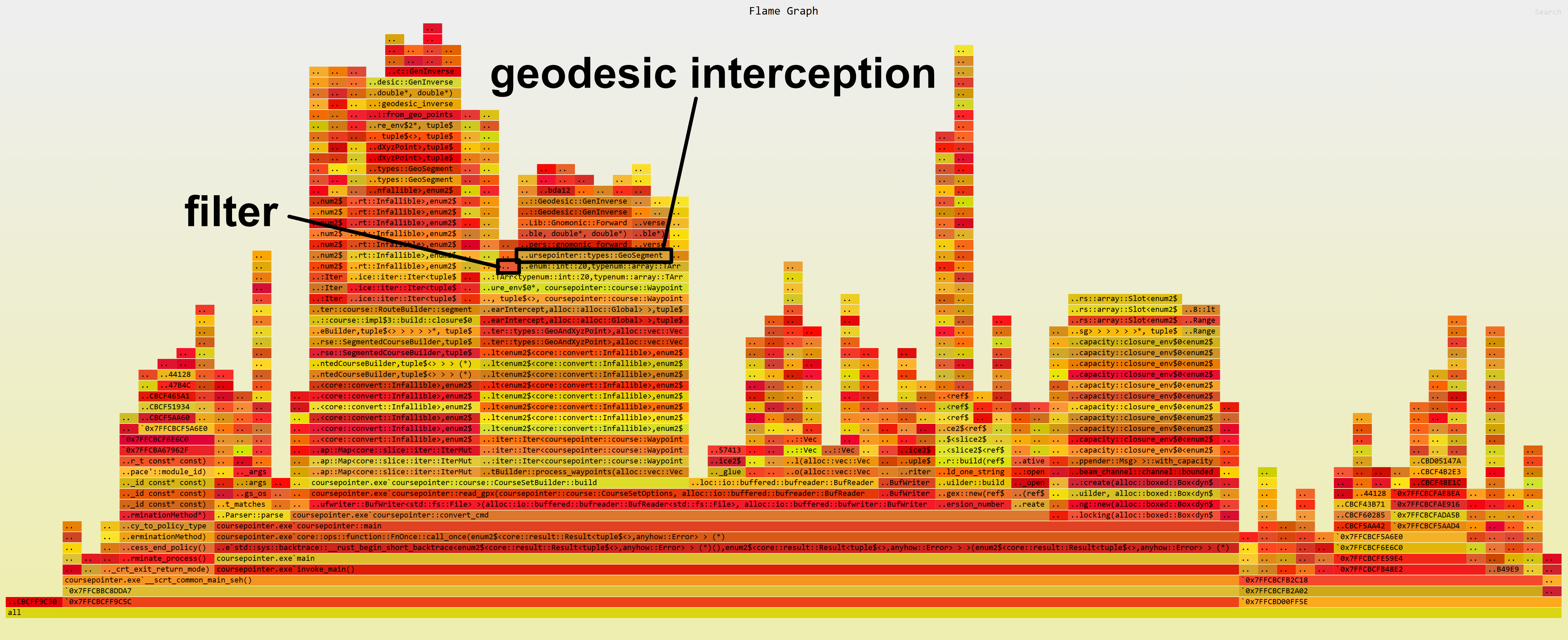
Figure 9: The time spent processing the example road cycling route on Windows with rayon disabled.
Performance counters in CoursePointer’s debug logs provide some useful context. For this course:
- 62,872 total waypoint-segment combinations were processed (29 waypoints times 2168 nonzero segments)
- 91 combinations passed the Euclidean filter and required computing a geodesic interception
- Of those 91, none were false positives that got rejected as out-of-threshold by geodesic interception after having been accepted by our filter
For this real-world course the filter is extremely selective, yet it’s still the geodesic algorithm that dominates the overall time spent calculating interceptions. This tells us that trading selectivity for higher performance in the filtering stage would be a bad choice, at least for routes of typical length. Instead, any additional improvements would likely be found by either improving the performance of my geodesic interception implementation, or by further reducing the total number of geodesic interceptions that must be computed.
Correctness
To double-check the filter’s correctness on top of the mathematical argument above, I used a Sobol sequence to verify the filter invariant against actual geodesic interception at 10 million arbitrary points in the five-dimensional space of segment latitude, segment azimuth, segment length, point azimuth, and point displacement, in various ranges of segment lengths and waypoint offsets: up to 10 m, up to 10 km, and up to 10,000 km.
I’ve not done a numerical error analysis on the filter’s floating-point math; for now I simply add 1 μm of “padding” to the intercept floor to provide a safe margin of error.
Future Work
I’m still naively using ten iterations of the gnomonic approximation to calculate geodesic interceptions, as suggested by Karney in a SourceForge comment. The number of iterations performed could be reduced by adaptively responding to the algorithm’s convergence, and early testing shows this might reduce the amount of time spent on geodesic interception by around 75% while preserving a high-precision result.
I could also do more to reduce the number of segment-point combinations for which any geodesic interception is computed. In many cases, a chord’s will be tight enough that it’s probably unambiguous which segment gets closest to a point even before we go geodesic; in those cases, we could use Karney’s algorithm solely between the point and that one segment, skipping the surrounding segments that also pass the filter.
And finally, even though the filter is not currently the bottleneck, it would be fun to try a SIMD implementation to see how much of a speed-up we could achieve on extremely large inputs.
Summary
CoursePointer’s Euclidean filter algorithm is simple to implement, and it’s performant in practice for common types of routes. Working in 3D Euclidean space turns out to be great for bypassing the edge cases of a 2D projection while keeping the math simple and fast.
I haven’t done a rigorous performance comparison against implementations based on R-trees, nor against other filters using spherical approximations or 2D projections. The outcome of any such comparison would depend on the exact scale of routes and waypoints being tested, which will vary from one problem space to another. But the performance data I have for this algorithm suggests it’s an excellent choice for at least some practical tasks, and it’s probably a good first approach to try given its easy implementation without complex data structures.
The full interception algorithm is:
- Choose an interception threshold, such as 35 m. Route segments that approach a waypoint within this geodesic distance are considered “intercepted” by it.
- Convert each route point and waypoint into coordinates and store those alongside their latitude and longitude.
- Segment the route points into adjacent pairs and solve the inverse problem to get the geodesic distance between each pair. Also calculate the segment’s cumulative distance along the route, and its with and being the semi-major and minor axes of the WGS84 ellipsoid.
- For each waypoint, find its Euclidean distance from the chord between each segment’s endpoints. If that distance is greater than the threshold plus set the segment’s interception distance to infinity, otherwise use Karney’s algorithm to find its geodesic interception. If that distance is greater than the threshold, likewise set the segment’s interception distance to infinity; else, save the computed geodesic distance.
- Find the local minima of each waypoint’s sequence of segment interception distances and call those interceptions, then decide what you want to do with any waypoints that intercept a route multiple times.
Footnotes
| [1] | This is an evolution of my original approach in the Mathematica notebook [PDF] where I prototyped the algorithm. This post adds a tighter filter function for which I can provide a correctness proof (in contrast with my earlier hand-wavy version), plus measurement of the algorithm’s performance. I’m also posting this to make this solution more discoverable on the web, as opposed to in a Mathematica notebook hidden in a git repo. This new algorithm is not yet implemented in the latest CoursePointer release, but it is on main in the git repo. |
| [2] | Some terminology for people new to this problem space, as I was when I began this project: An oblate “spheroid” (or ellipsoid of revolution) is what you get if you take a circle, squish its top and bottom together a little, and then rotate it around its top-bottom axis into an ellipsoid. WGS84 is one specification of such an object, and it turns out to be a meaningfully more accurate model of Earth than any sphere. And the shortest path from point A to point B along the surface of that model is a geodesic. |
| [3] | This was all prompted by a long-standing bug in the Garmin Connect web app, since fixed, which had prevented the app from doing this correctly itself. That hindered creating routes with points of interest in GPX applications and having them appear as course points while navigating on my Edge bicycle computer. |
| [4] | You may have noticed this is the same calculation as finding the distance between a line segment and a point on a plane, except using 3D vectors. In my view this is a strong argument for doing this filtering phase in 3D space instead of a 2D projection: It eliminates the edge cases and other complexities inherent in a 2D projection, yet the math isn’t actually more complicated! |
| [5] | CoursePointer originally derived a maximum distance in terms of chord length, as based on a loose geometric argument, though I lacked a rigorous proof. From Lemma 3 in the same paper, we can obtain a maximum geodesic length for a chord length as Combined with Lemma 13, this gives us However, since we need to compute each segment’s geodesic length anyway in order to obtain the cumulative course distance, we can use Lemma 13 alone for a tighter bound. |
| [6] | This technically encloses a pill-shaped superset of the cylinder that also contains extra space around the chord’s endpoints, but it’s what I currently do in CoursePointer for simplicity’s sake. |
| [7] | I had trouble getting intercept_distance_floor to even register in a sampling profile on my Linux box. On this Windows machine, converting this same course takes a little longer overall, around 8.84 ms. While rayon is enabled in release builds of CoursePointer, I disabled it here for a slightly easier-to-read flame graph. |
References
| [8] | Earle, Michael A. “Sphere to Spheroid Comparisons.” Journal of Navigation 59, no. 3 (2006): 491–96. https://doi.org/10.1017/S0373463306003845. |
| [9] | (1, 2) Karney, Charles F. F. “Algorithms for Geodesics.” Journal of Geodesy 87, no. 1 (2013): 43–55. https://doi.org/10.1007/s00190-012-0578-z. |
| [10] | Baselga, Sergio, and José Carlos Martínez-Llario. “Intersection and Point-to-Line Solutions for Geodesics on the Ellipsoid.” Studia Geophysica et Geodaetica 62, no. 3 (2018): 353–63. https://doi.org/10.1007/s11200-017-1020-z. |
| [11] | C. F. F. Karney, GeographicLib, Version 2.7 (2025-11-06), https://geographiclib.sourceforge.io/C++/2.7 |
| [12] | Boissonnat, Jean-Daniel, André Lieutier, and Mathijs Wintraecken. “The Reach, Metric Distortion, Geodesic Convexity and the Variation of Tangent Spaces.” Journal of Applied and Computational Topology 3, nos. 1–2 (2019): 29–58. https://doi.org/10.1007/s41468-019-00029-8. |